library(mizerExperimental)
library(mizerMR)
library(tidyverse)

# Load tuned model with original selectivity
cm <- readParams("cur_model_resilient.rds")Change resources
Introduction
Mizer can be used to explore the consequences of climate change on aquatic ecosystems and fisheries. One of the major effects that climate change is having on aquatic ecosystems is a change in plankton and benthos abundance and size structure. However, responses in resources are highly uncertain and variable and predictions are difficult. For plankton we can use satellite observations of chlorophyll A and earth system models to assess past changes and aim to predict the future. Benthos changes also are likely having large impacts on shallow water ecosystems, but in many cases we have almost no empirical data on how much change is happening. Nevertheless we might want to explore the potential effect of these changes on the rest of aquatic food webs and on our fisheries. This is what we are going to do in this tutorial.
As usual we load libraries and also load the parameter file from the first tutorial, where we tuned the reproduction parameters.
Resource dynamics
Let’s look at the resource parameters once again
resource_params(cm)We see four main resource parameters that we already met in the tutorial on multiple resources: we already know kappa, which defines the overall abundance of the resource, and lambda, which is the slope of the resource spectrum. We also know w_min and w_max, which set minimum and maximum resource sizes.
For people who have already been using mizer to build or tune models in the past we need to draw attention to a change in the meaning of these resource parameters.
In the past, the parameters were used to set the resource carrying capacity, i.e., the hypothetical resource abundance that would be realised if there was no consumption by fish. In the new version, the parameters are used to set the actual observed resource abundance, in the presence of consumption by fish.
In the old version of steady(), the resource abundance would change during the tuning of the model. This made tuning of the model more difficult, especially if one wanted to reproduce observed resource abundances. The new version of the steady() that we used while tuning the model is keeping the resource abundance fixed and then adjusts the resource carrying capacity. So now the hypothetical carrying capacity is the emergent quantity and the observed abundance is specified by the resource parameters.
Sheldon’s spectra in natural ecosystems reflect abundances in natural systems and not a hypothetical carrying capacity that would emerge if there was no feeding on the resource. It makes sense to use the resource parameters to specify an observable quantity rather than a hypothetical one.
This is not really a breaking change, because all existing mizer models will continue to work in the same way as in the past. The change only affects the tuning of a model with the steady() function.
We will now explain the parameters r_pp and n.
Note that the resource dynamics are very different from the size-spectrum dynamics for fish because there is no growth between sizes classes. There is only birth and death, independently in each size class. The abundance in a size class is the result of the balance between the birth and death rates in that size class. So we can understand the dynamics for each size class separately. We just have to understand how the birth and death rates are determined.
Semi-chemostat resource dynamics means that the total birth rate decreases as the resource number density N_R(w) gets closer to its carrying capacity c_R(w), in such a way that the total birth rate at size w is given as (c_R(w) - N_R(w))r_R(w). We refer to r_R(w) as the intrinsic replenishment rate or just the resource rate. Stated the other way around: as the resource abundance drops, its birth rate increases. This is essential for the resilience of the system to perturbations as we will explain below.
The parameters r_pp and n are used to set the intrinsic replenishment rate r_R(w) of the resource to an allometric power law
r_R(w) = r_{pp}w^{n-1}.
The default choice for the exponent n is 3/4, so that the replenishment rate decreases with size. Smaller resource size classes can replenish faster than larger size classes.
The resource is consumed by fish in proportion to its abundance. So the total death rate at size w is \mu_R(w)N_R(w) where \mu_R(w) is the per-capita mortality rate. This mortality rate on resource is determined by predation by fish in the same way as the mortality rate on other fish. So a higher abundance of fish leads to a higher mortality of resource.
In the steady state, the birth and death rates are in perfect balance. But if the fish abundance increases and thus the resource mortality rate increases, the resource abundance goes down. However, because the resource birth rate increases as the resource abundance goes down, a new steady state is soon established. The semi-chemostat dynamics are stable.
By definition, the steady state resource number density N_R will always be below the resource carrying capacity c_R. We refer to the ratio N_R / c_R as the the resource level. This has to be a number between 0 and 1. This is similar to the feeding level and the reproduction level.
How much the steady state resource abundance N_R changes when the predation mortality from fish increases depends on the resource level. This is best illustrated by a diagram.
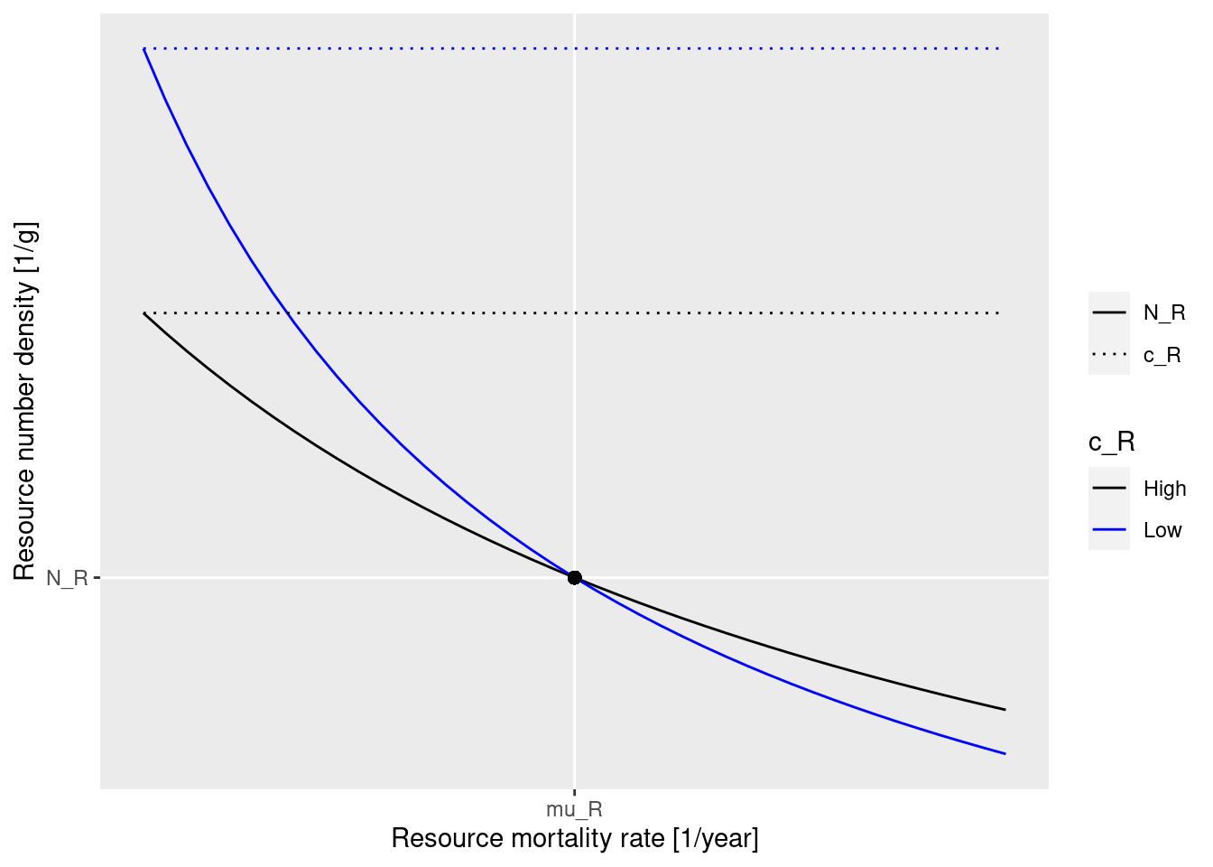
The black dot represents the steady state situation, the one we have tuned our model to. The solid lines show how the resource abundance on the y axis will change as the resource mortality on the x axis changes away from the steady state value. The blue line gives the relationship for a higher carrying capacity, the black line gives it for a lower carrying capacity. We see that for a given change in the resource mortality, the change in resource abundance is larger along the blue curve than along the black curve. So the blue curve corresponds to more sensitivity of the resource to changes in the fish abundance and the black curve corresponds to more resilience of the resource. The blue curve is for a resource level of 1/3 and the black line for a resource level of 1/2. The closer the resource level is to 1 the shallower the curve and the more resilient the resource.
Just like with reproduction level, we did not need to worry about resource level while we were tuning the steady state because the steady state does not change as the resource level changes. But the resource level becomes important when we investigate perturbations away from the steady state.
We do not set the resource level directly. We set the replenishment rate r_R and this determines the resource level:
{\tt resource\ level}(w) = \frac{r_R(w)}{r_R(w) + \mu_R(w)}.
So the resource level depends both on the replenishment rate and on the predation mortality that the fish exert on the resource.
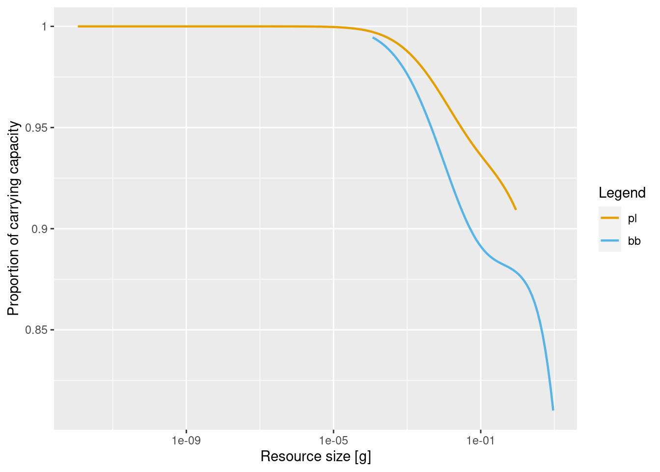
Let’s look at the resource level in our model.
The resource level is close to one for the smaller resource because almost no fish consume it, but the resource level drops for larger resource.
Scenario 1: Changes in resource replenishment rate
We will now change the resource replenishment rate for plankton to see how that affects the resource level for plankton and how that affects the system’s response to changes in fishing. We change the value of the r_pp for the plankton resource and choose the two values 10 and 1 for the high and the low replenishment rate.
# Create new data frame for high and low plankton replenishment
rp <- resource_params(cm)
rp_Pl_high <- rp
rp_Pl_high["pl", "r_pp"] <- 10

rp_Pl_low <- rp
rp_Pl_low["pl", "r_pp"] <- 1
We will use a new function setResourceSemichemostat() to update resource parameters.
cm_Pl_high <- setResourceSemichemostat(cm, rp_Pl_high)

cm_Pl_low <- setResourceSemichemostat(cm, rp_Pl_low)The setResourceSemichemostat sets the resource carrying capacity so that the resource abundance is at steady state with the given replenishment rate and the mortality rate exerted by the current fish abundances. This means that if we start with a steady state of the whole system and only change the replenishment rate by changing the r_pp and/or n parameters, then the steady state is preserved. However, if we change the resource abundance by changing the kappa, lambda, min_w or max_w parameters, this changes the food available for the fish and thus their growth rates. This means that the fish spectra will change over time and thus the resource mortality rate will change and the resource will no longer be at steady state. We’ll see an example of that in the next scenario.
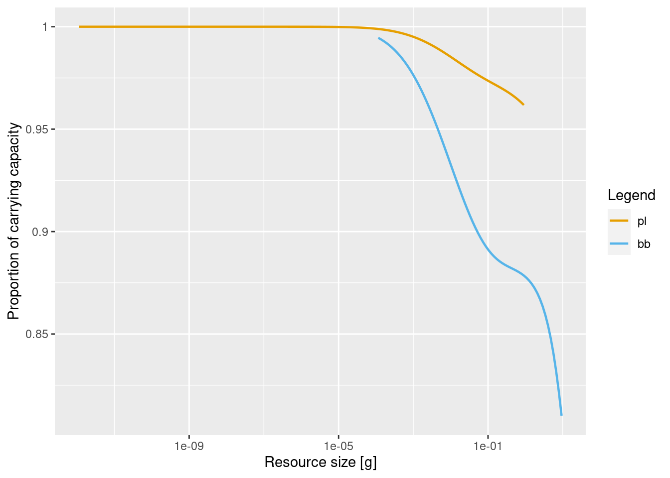
Let us look at the changed reproduction levels:
plotResourceLevel(cm_Pl_low)
plotResourceLevel(cm_Pl_high)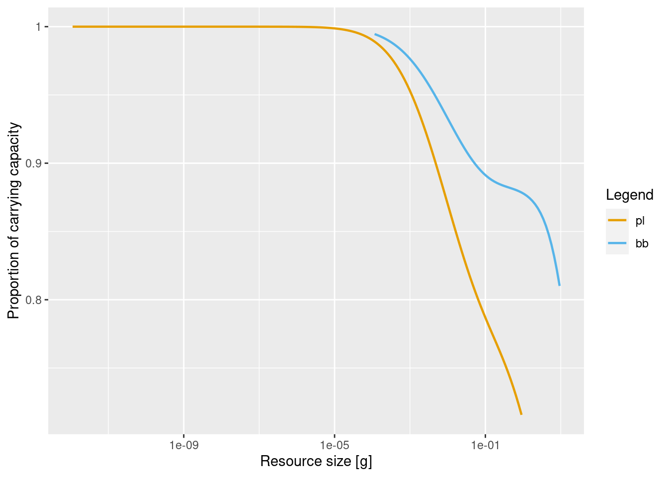
The changed resource level should lead to differences when we perturb the system away from its steady state. We will perturb the system by imposing a higher fishing effort.We will run simulations with the reduced and the increased replenishment rate with a fishing effort of 0.7. As a result of that higher fishing effort, the fish biomasses will change and hence resource consumption will change. The resource level will determine how sensitive the system is to that change.
# Lower replenishment, higher effort
sim_lower <- project(cm_Pl_low, effort = 0.7, t_max = 50)
plotlyBiomassRelative(sim_lower)
# Higher replenishment, higher effort
sim_higher <- project(cm_Pl_high, effort = 0.7, t_max = 50)
plotlyBiomassRelative(sim_higher)
low plankton replenishment
high plankton replenishment
The differences in the response of the system to the higher fishing effort are not very different for the two different resource replenishment rates. To see the differences better we plot their relative difference.
plotlyBiomassRelative(sim_lower, sim_higher)We can see that in this case the differences are never much more than 4%, which is very little considering all the uncertainties in the model. We conclude that for our model, when we want to explore increases in fishing effort, the choice of value for r_pp may not be so important, as the model is not very sensitive to it. However, that may be an artefact of how we have set up external mortality in our model. In our model, mortalities on small individuals are very low and we didn’t bother to fix them with additional mortality to get the allometric mortality rates observed in nature. Had we done that, even small changes in the resource and hence in the larval feeding levels might be important. This is because lower feeding by larvae will make them grow slower, they will spend more time in smallest size classes with very high mortality, and this will affect the entire ecosystem. You can read about it, in this study. And if you want to explore it further and implement it to your model, the mizer code is here.
Exercise
Now reduce the replenishment rate coefficient r_ppon both plankton and benthos to just 0.01. In addition, increase the fishing effort from 0.3 to 0.4 and project the model far enough to reach a new steady state. By how many percent approximately is the biomass of roach higher in this new steady state than in the original one?
There will be no further formal exercises for you to complete, but of course we hope that you will feel the urge to do your own explorations of other scenarios.
Scenario 2: Changes in total plankton abundance
Now we want to explore how our ecosystem might respond to the overall changes in resource abundance. Perhaps due to climate change the overall resource abundance will increase or decrease. We can explore this in a simple way by changing the kappa parameter.
Now we will change plankton kappa in the same way as we changed r_pp in the previous scenario. Just to make sure we see some impact, let’s increase or decrease kappa by 50% and project to a new state.
# Create new resource parameter data frames for more and less plankton
rp_more_be <- rp
rp_less_be <- rp

# Increase kappa by 50%
rp_more_be["pl", "kappa"] <- rp_more_be["pl", "kappa"] * 1.5

# Decrease kappa by 50%
rp_less_be["pl", "kappa"] <- rp_less_be["pl", "kappa"] / 1.5

# Put new the resource parameters into the models
cm_more_be <- setResourceSemichemostat(cm, rp_more_be)

cm_less_be <- setResourceSemichemostat(cm, rp_less_be)
Let’s check that resource abundances really changed by plotting the spectra
plotSpectra2(cm_more_be, "More", cm_less_be, "Less", power = 2)
As we discussed before, while the setResourceSemichemostat() has set the resource carrying capacity so that initially the new resource abundance is steady, the fish abundances will change over time in response to the changed resource abundance and as a result also the resource abundance will start to change. Let us investigate that by projecting for 50 years with the new level and compare to the unchanged conditions.
sim_more_plankton <- project(cm_more_be, t_max = 50)
plotlyBiomassRelative(sim_more_plankton)
sim_less_plankton <- project(cm_less_be, t_max = 50)
plotlyBiomassRelative(sim_less_plankton)
more plankton
less plankton
These results are quite expected. As plankton abundance increased, biomasses and yields for all species also increased. Roach benefited most, but pikeperch was also affected positively. Predator_fish also increased. The effect of decreasing plankton abundance is strongest on roach, pikeperch and predator_fish. So the overall effects of 50% increase and decrease in plankton kappa are rather symmetrical and expected.
Let us also look at the feeding levels in the new steady states
plotlyFeedingLevel(sim_more_plankton)
plotlyFeedingLevel(sim_less_plankton)
more plankton
less plankton
As expected, the feeding level for small individuals, which rely most on plankton for their food, are lower for lower plankton abundance.
Scenario 3: Changes in total benthos abundance
From the plankton exercise we might expect that changing benthos will lead to similar ecosystem change. But this is not necessarily the case, because all species feed on plankton, yet only some species feed on benthos. Without exploring this question in a multi-species context, we cannot really predict. We will follow exactly the same steps as in the previous scenario.
# Create new resource parameter data frames for more and less plankton
rp_more_be <- rp
rp_less_be <- rp

# Increase kappa by 50%
rp_more_be["bb", "kappa"] <- rp_more_be["bb", "kappa"] * 1.5

# Decrease kappa by 50%
rp_less_be["bb", "kappa"] <- rp_less_be["bb", "kappa"] / 1.5

# Put the new resource parameters into the models
cm_more_be <- setResourceSemichemostat(cm, rp_more_be)

cm_less_be <- setResourceSemichemostat(cm, rp_less_be)

# Check on the spectra plot that the changes have taken place
plotSpectra2(cm_more_be, "More", cm_less_be, "Less", power = 2)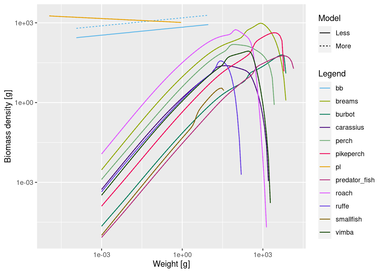
Now we will project for 50 years with the new level and see how the biomasses are changed
sim_more_be <- project(cm_more_be, t_max = 50)
plotlyBiomassRelative(sim_more_be)
sim_less_be <- project(cm_less_be, t_max = 50)
plotlyBiomassRelative(sim_less_be)
more benthos
less benthos
Surprisingly, the effects of decreasing benthos are far less pronounced on benthivorous fish, like roach, carrasius and breams. And it is perch and pikeperch that increased most, when benthos increased. It appears that benthivorous species were affected by changes in their predators and this counteracted the changes in their growth rate that are caused by the changes in their benthic resource.
This is just a simple exploration, but it demonstrates that in a multi-species system that consists of different trophic groups (planktivores, benthivores, predators), changes in plankton and benthos resource levels can have different and sometimes unexpected effects on species and yields. Also, different resources are likely to respond to climate change differently, and mizerMR provides an opportunity to explore it. Remember, you can set more than two resources in mizerMR. In fact, every species could have its own resource, although this would be a pretty boring model. But if you have a good reason to set 3 or 4 separate resources, this can be easily done.
Scenario 4: changes in resource size structure and replenishment rate
It has also been suggested that climate change is changing the size structure of aquatic organisms, from plankton to fishes. We can attempt to model such changes in resource size structure by changing the lambda parameter. Mostly, it is expected that organisms will get smaller, so we expect lambda to become steeper (have larger values). But at the same time benthic organisms might have faster growth rates, so their sizes might increase. These are just entirely hypothetical scenarios, but we can explore how potentially different responses in plankton and benthos will affect the ecosystem. But unlike with kappa we change lambda just by a small amount, because even small changes in allometric exponents will have large effects on the size spectrum.
We will repeat the steps from above - save the dataframe, update it with new parameters, check, put it back into params objects:
# Create new resource parameter data frames for more and less plankton
rp_steeperPl <- rp
rp_shallowBe <- rp
rp_Both <- rp

# Increase plankton lambda by 0.1, setting it to 2.15 instead of 2.05
rp_steeperPl["pl", "lambda"] <- 2.15
# Decrease benthos slope by 0.1, setting it to 1.8
rp_shallowBe["bb", "lambda"] <- 1.8
# And now make both changes
rp_Both["pl", "lambda"] <- 2.15
rp_Both["bb", "lambda"] <- 1.8

# Put the new resource parameters into the models
cm_steeperPl <- setResourceSemichemostat(cm, rp_steeperPl)
cm_shallowBe <- setResourceSemichemostat(cm, rp_shallowBe)
cm_Both <- setResourceSemichemostat(cm, rp_Both)
Now we project with steeper plankton slope for 50 years and look at the relative changes in the biomasses.
sim_steeperPl <- project(cm_steeperPl, t_max = 50)
plotlyBiomassRelative(sim_steeperPl)
Here changes are more dramatic, with all species increasing their biomases with steeper plankton slopes. This might sound strange and counter intuitive, but we must realise that slope only affects the steepness of the resource, keeping abundance at 1g constant. So steeper slopes mean less plankton larger than 1 g, but more plankton small than 1 g. And since our maximum plankton size is only 1g, we only increased its abundance!
Now let’s look at the effect of changes in the benthos slope.
sim_shallowBe <- project(cm_shallowBe, t_max = 50)
plotlyBiomassRelative(sim_shallowBe)
With more shallow benthos slopes, roach and pikeperch are affected badly and other benthivores decrease slighly, but are probably benefiting from reduced predation due to reduced predator biomass. We can compare feeding level changes and see that large predators have largest decreases in feeding level.
plotlyFeedingLevel(sim_steeperPl)
plotlyFeedingLevel(sim_shallowBe)
steeper plankton
shallower benthos
And what happens if both plankton and benthos slopes change?
sim_Both <- project(cm_Both, t_max = 50)
plotlyBiomassRelative(sim_Both)
Now effects partly balance each other out, but to understand this better we will compare to simulations where, for example, only plankton slope changed. This can help isolate the interacting effects.
plotlyBiomassRelative(sim_Both, sim_steeperPl)
plotlyYieldRelative(sim_Both, sim_steeperPl)
Biomass
Yield
You can also try to combine these changes in lambda with changes in the resource replenishment rate (which can either go up or down due to climate change) and see how many options we already have. And then these lambda changes will probably also interact with changes in kappa, and feed back into the ecosystem through species interactions. Moreover, our system response to these changes will depend on reproduction level and resource resilience parameters (replenishment rate), and it will depend on other parameters for our species. This gets complicated very quickly. On top of that we probably want to explore how fishing might interact with changes in the resource abundance, so that gets even more complicated. This is not to discourage you, but to show that there are plenty of opportunities for exploration and interesting publications. We are still very uncertain on how resources will respond to changes in climate and will probably learn a lot more in the future.
Scenario 5: Changes through time
The scenario explorations above were very simple, because we changed one or several of resource parameters and projected the system to a new steady state. While the mechanics of setting such scenarios is straightforward, examples above show that understanding all the complex ways how simple changes can affect the ecosystem may be harder.
However, many researchers do not want to explore such hypothetical resource changes, but instead use independently derived time series of resource abundance provided by e.g. satellite observations and earth system models. This is important and useful, although we do encourage you to play with simple changes first to gain understanding about your system and its sensitivity to resource changes. Just like with fishing mortality scenarios, ecosystem response will depend strongly on our model calibration. This means that before we go into complex scenarios we need to be satisfied with the parameters we provided and know limitations of our simulations. For example, alternative, equally possible model calibrations may provide different quantitative change (i.e. how much the biomasses or yields change), but similar qualitative response in the ecosystem. If quantitative differences are very large, perhaps it would be best to focus on more general qualitative responses.
But let’s look at how we can implement multiple drivers under climate change by coupling mizer to outputs of earth system models such as temperature, abundance of different size classes of plankton or detrital “marine snow” that reaches the sea floor through time. This example is provided by Julia Blanchard and it demonstrates how to implement changes in resource abundance and size structure through time, by working with pre-made resource size spectra files that were estimated from two climate change scenarios from earth system model output.
These resource spectra files were derived from small and large phytoplankton biomasses predicted by the Fisheries and Marine Ecosystems Model Intercomparison Project (FishMIP). There are a lot of steps in processing these data, but we won’t go in to that here. The main goal is to demonstrate how to use these scenario forcings to create changes in your mizer resources through time. This example will use another model - Patagonian toothfish fishery ecosystem. We will explore how the marine demersal fish community changes under this forcing through time. The two model scenarios are ssp585 (highest emissions or “worst”) and ssp126 (mitigation to cut emissions or “best”). Note: this new model does NOT use multiple resources
Read in the model and the resource abundances provided by the earth system model.
download.file("https://github.com/sizespectrum/mizerCourse/raw/main/use/toothfish_model.rds",
              destfile = "toothfish_model.rds")
download.file("https://github.com/sizespectrum/mizerCourse/raw/main/use/resource_scenario_126.rds",
              destfile = "resource_scenario_126.rds")
download.file("https://github.com/sizespectrum/mizerCourse/raw/main/use/resource_scenario_585.rds",
              destfile = "resource_scenario_585.rds")
params <- readParams("toothfish_model.rds")
resource_best <- readRDS("resource_scenario_126.rds")
resource_worst <- readRDS("resource_scenario_585.rds")The data files provide arrays with dimensions time x size with the resource number density in the years from 2021 to 2070 for all size classes in the model, as predicted by the earth system model.
str(resource_best) num [1:50, 1:209] 7.34e+31 7.98e+31 7.90e+31 7.53e+31 7.65e+31 ...
- attr(*, "dimnames")=List of 2
..$ : chr [1:50] "2021" "2022" "2023" "2024" ...
..$ : chr [1:209] "9.42976673097891e-13" "1.14104741933864e-12" "1.38072260992634e-12" "1.67074119204156e-12" ...We now create new mizer models that contain this information about the plankton abundance. Mizer allows us to add an arbitrary number of other parameters to the model. We decide to call our new parameter resource_array.
#create new params files
params_worst <- params
params_best <- params

# Add extra `resource_array` parameter to these model
other_params(params_best)$resource_array <- resource_best
other_params(params_worst)$resource_array <- resource_worst
Instead of running mizer’s standard resource dynamics we want the resource abundance to be taken from these arrays. To achieve this we will use a handy mizer feature that allows us to provide our own resource dynamics function. That function just needs to return the value for the resource at the next time step. So in our case it just needs to look up the correct value in an array.
plankton_forcing <- function(params, t, ...) {
    # The time `t` will run from 2021 to 2070 whereas the time index in the
    # array runs from 1 to 50. Hence we need to index by t - 2020.
    # In fact `t` will take on fractional values like 2021.1 after the first
    # time step, but R conveniently rounds them down automatically.
    other_params(params)$resource_array[t - 2020, ]
}
Now we just have to register this new function as the resource dynamics function in the models:
params_best <- setResource(params_best, resource_dynamics = "plankton_forcing")
params_worst <- setResource(params_worst, resource_dynamics = "plankton_forcing")
This means that in each time step the resource abundance (only plankton in this case, as this is the only resource in this model) will be determined not by the semi-chemostat dynamics, but by the externally provided values.
Now we will project these new models forward for 50 years from 2021 to 2070 without fishing.
Let’s look at how the biomasses evolve in these models:
plotlyBiomassRelative(sim_best)
plotlyBiomassRelative(sim_worst)
Best
Worst
This shows how the effects of plankton changing alone can have a big effects on the model.
animateSpectra(sim_worst, power = 2)This example has shown how you can directly use outputs of earth system models for projections (GFDL inputs - FishMIP).
Summary
- The resource replenishment rate coefficient
r_ppwill determine the resilience of the resource spectrum to mortality imposed by fish. In many scenarios, the choice of replenishment rate may not make a big impact, but in others it will be important. Therefore we should explore how this parameter might affect our model dynamics (together with other parameters, of course). - Climate change is likely to impact resource abundance, size structure and productivity. Mizer allows you to explore how these changes might impact aquatic ecosystems and yields.
- By separating plankton and benthos resource mizerMR allows us to model separate resource responses to climate, which are likely to lead to different responses in different trophic groups of fish. There are many potential ways how these resources can change, so one needs to carefully consider how best to select scenarios.
- We can change resource dynamics to functions other than semi-chemostat. Mizer allows you to force models with externally obtained resource time series. This way we can explore gradual ecosystem changes through time.
Further explorations and climate change effects
If you want to explore how changes in the resource due to climate change can affect ecosystems with multiple resources you can look at two recent model applications. One example is a recently published Baltic Sea mizer model where authors explored how changes in resource total abundance (kappa) and replenishment rate (r_pp) might affect the ecosystem.
Another example in the Tasmanian rocky reef model (a preprint can be found here), where authors used multiple parameter combinations to assess how changes in kappa and lambda for plankton and benthos might affect the ecosystem. The Tasmanian model has a supporting R Shiny application that allows you explore your own resource change scenarios, using one parameterisation. Here you can change kappa and lambda of either plankton or benthos resource and combine resource changes with physiological responses to temperature change, by also changing model temperatures. This will display changes in biomass, yields and mean sizes for the modeled fish species.
Despite all the complexities above, we barely scratched the surface about the possible ways how climate change might affect our ecosystems. For example, so far we did not include any direct temperature effects. Even though we modeled resource change, this was imposed externally and did not combine with possible effects of temperature on physiology. If you want to also include temperature effects on fish physiological rates, take a look at the excellent blog post by Phoebe Woodworth-Jefcoats in the mizer blog. She describes how you can replace rate functions in mizer with your own set functions and she uses this to account for dome-shaped species responses to temperature - increased rates up to a certain temperature and decreases after that.
Of course climate change will also affect the composition of species, because with warming new species will enter the ecosystem. This is an important aspect to address, but has not been thoroughly explored yet. Mizer allows you to add new species into ecosystem with the addSpecies() function. However, it is not necessarily clear how we tune parameters of new species for which we don’t yet have data (in that ecosystem at least), so exploring climate heating driven species composition change is not straightforward.
